Monte Carlo & Historical Analysis (Available in Unlimited Plan)
1. “All models are wrong, but some are useful.”
— George Box
This quote should ALWAYS be kept in mind. We create models and run analysis to provide the outline of a picture, to validate broad assumptions — or to alert us of potential danger. No matter how painstakingly detailed our assumptions are, there are no guarantees the results will be 100% accurate.
To give you the most complete view we can, OnTrajectory provides three different strategies for modeling growth in your investments.
1. Average Growth — This is the default technique employed when setting up and configuring your Trajectory. It is dictated by the % Growth field for each account. The advantage of this technique is that you can fine-tune your Trajectory and easily visualize the result of small changes over long periods of time.
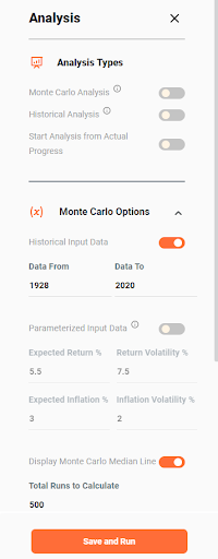
2. Monte Carlo — This type of analysis provides the likelihood that your Trajectory will be defined as 'successful' (i.e. you didn't run out of cash). It is based either on randomized historical data or data parameters that you define, which then replaces % Growth and Inflation. See below as an example of how to customize your analysis:
Unlike Average Growth, which produces a single Trajectory line, Monte Carlo produces a range of results because multiple randomizations ('Total Runs') are calculated for every year of your Trajectory. See the section Running Monte Carlo Analysis below for more information.
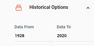
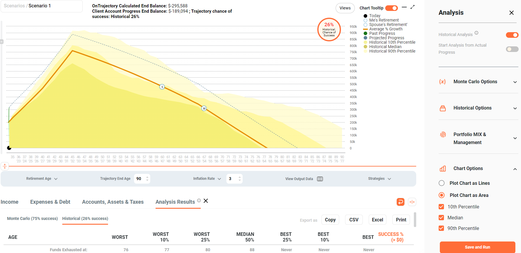
3. Historical — This type of analysis uses only historical data. Unlike Monte Carlo, however, data is not chosen randomly, but rather sequentially. In other words, for Year 1 data from 1928 is used, for Year 2 data from 1929 is used, for Year 3 data from 1930 is used, etc. In addition, a sequential run is created for every year in the range. For example, a sequence starting Year 1 in 1928, then a sequence starting Year 1 in 1929, etc.
See below as an example of how the year range can be set up:
Since we calculate results for every available year in the year range, we can produce a success percentage similar to that for Monte Carlo analysis. See the section Running Historical Analysis below for more information.
2. Running Monte Carlo Analysis
When OnTrajectory runs Monte Carlo analysis, we take into account every Income, Expense and Account you have defined — along with every RMD, drawdown, rollover, gain, tax or penalty calculated along the way. Every aspect used to render your Trajectory is recalculated for each individual Monte Carlo 'run'.
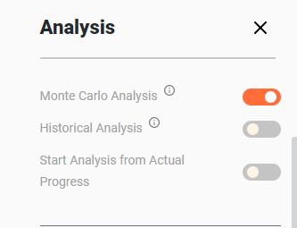
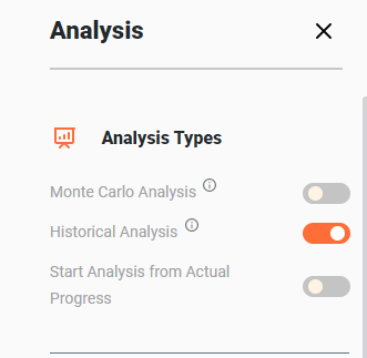
To initiate Monte Carlo analysis, select ‘Analysis’ from the Strategies dropdown menu. Toggle the Monte Carlo button to ‘On’ and the analysis will start.
If you wish to customize the data that is being run, open the Monte Carlo Options window and select the options you would like to change and press the save and run button. See screenshot below:
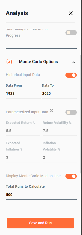
As discussed above, Historical Input Data simply draws randomly from a set of years as defined in the "Data From:" and "Data To:" fields. Parameterized Input Data, on the other hand, allows you to set both an Expected Return (expected average annual return) and Expected Inflation (expected average annual inflation) — as well as Volatility (standard deviation) for each.
The following tables list historical annualized returns and volatility for various time periods and portfolio mixes that may be used while running simulations ("Equity" is the S&P 500 Index and "Bond" is the Five Year Treasury Note):
| From 1929 to 2018 | Annualized Return % | Annualized Volatility |
| 100% Equity / 0% Bond | 10.2 | 18.6 |
| 80% Equity / 20% Bond | 9.5 | 14.8 |
| 60% Equity / 40% Bond | 8.6 | 11.2 |
| 40% Equity / 60% Bond | 7.6 | 7.9 |
| From 1970 to 2018 | Annualized Return % | Annualized Volatility |
| 100% Equity / 0% Bond | 10.5 | 15 |
| 80% Equity / 20% Bond | 10.1 | 12.1 |
| 60% Equity / 40% Bond | 9.5 | 9.4 |
| 40% Equity / 60% Bond | 8.8 | 7.0 |
| From 2000 to 2018 | Annualized Return % | Annualized Volatility |
| 100% Equity / 0% Bond | 5.6 | 14.4 |
| 80% Equity / 20% Bond | 5.8 | 11.0 |
| 60% Equity / 40% Bond | 5.7 | 7.9 |
| 40% Equity / 60% Bond | 5.5 | 5.2 |
*Above data is from the "Returns" program, Dimensional Fund Advisors (DFA).
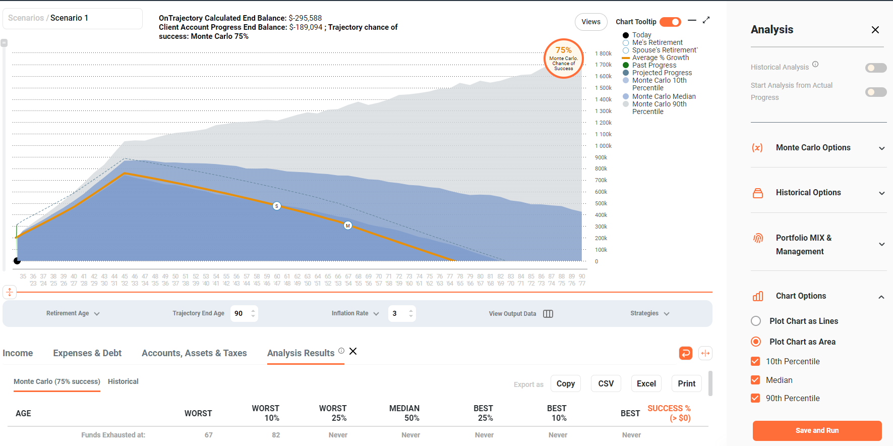
Further down this window, you can choose to view the Monte Carlo analysis as plotting the chart as ‘Area’ or as ‘Lines’. See the two screenshots below:
Plotted Area
Plotted Lines
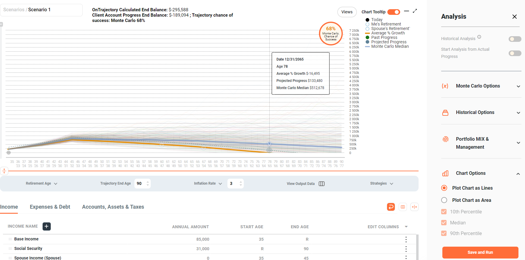
Because multiple Monte Carlo cycles are run, multiple results are displayed. Your Trajectory is displayed in orange, along with a "success" percentage. This percentage represents the number of simulated runs that ended above $0. In other words, for the example above, 68% of the simulated runs ended with some amount of money left over. In 32% of them, you ran out of cash.
Optionally, you can display the 'Median' Monte Carlo Trajectory (displayed in blue), meaning there is an equal number of Monte Carlo runs above and below it.
3. Running Historical Analysis
Just like Monte Carlo analysis, Historical analysis takes into account every Income, Expense and Account — along with every RMD, drawdown, rollover, gain, tax or penalty calculated along the way.
To initiate Historical analysis, select ‘Analysis’ from the Strategies dropdown menu. Toggle the Historical Analysis button to ‘On’ and the analysis will start.
If you wish to customize the data that is being run, open the Historical Analysis Options window and select the options you would like to change and press the save and run button. Changing the years of data dictates how many runs will be completed (based on the length of your model). For example, if your model goes from age 40 to 90, 50 years are needed for a complete run. If you are using data that begins in 1928, the final year of the analysis for the first run will end in 1978. For run two, the data will span 1929 to 1979 -- for run three, 1930 to 1980, etc. If the final year of data is 2020, the last run will begin in 1970, since there is not enough data for a complete run starting in 1971.

As with Monte Carlo, you can choose to view the Historical Analysis either as plotted areas or lines.
Example of Historical Analysis as plotted area:
4. Portfolio Mix / Management
Above we stated that for both Historical and Monte Carlo analysis, "% Growth" and "Inflation" can be based on historical data, but which particular data are we talking about — and how is that data applied?
The "Portfolio Mix / Management" tab defines the percentage of each Investment Type (Stocks, Bonds, Cash) in your virtual portfolio for when historical data is used (as shown below).

Adjust the mix to your liking, but be careful. Although the default settings seem to take a very conservative approach, remember that when using Historical data, all Accounts get identical rates-of-return for a particular year — and this includes whatever funds you have in low-yield accounts as well as excess income you may not have invested. Our default ratio is similar to those used by other simulation tools.
The underlying data comes from a variety of sources:
- Stocks — based on S&P 500 Index,
- Bonds — based on 10-Year Treasury Bond Index,
- Cash — based on a 3-Month Treasury Bill Index.
- Inflation — based on Consumer Price Index (CPI-U) compiled by the U.S. Bureau of Labor Statistics.
Finally, "Management Expense Fee" represents a burden to your growth rate based on fees you may pay to an advisor or for other management costs. If populated, this percentage is subtracted from the growth rate in each account in each simulated year, regardless whether Historical or Parameterized input data is chosen. If you feel that you are experiencing better than market returns as a result of having assets under management, do NOT enter a Management Fee.
5. Factors Affecting Growth
As you experiment with different year ranges, portfolio mixes, or input parameters — you will see how your Trajectory is affected by factors such as Variance Drain (i.e. overall lower returns produced by periods of high volatility) and Sequence Risk (i.e. long-term lower performance when market declines occur at the beginning of an investment period). We recommend using sites such as Investopedia to understand how these and other various factors affect your investments.
6. Viewing Results
- The Worst run
- Worst 10%
- Worst 25%
- Median 50%
- Best 25%
- Best 10%
- The Best run
- Success % — the percentage of runs that stayed and ended greater than 0.
An example of Analysis Results is shown below:
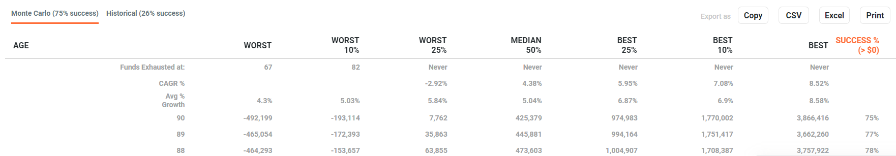
The CAGR % row displays the Compound Annual Growth Rate for the group represented by a particular column. It can be thought of as the growth rate that gets you from the initial investment value to the ending investment value if you assume that the investment has been compounding over the time period. In a scenario where either the initial Trajectory balance or the ending Trajectory balance is negative, it is not possible to compute CAGR % — you will see a blank entry to represent such an occurrence.
The Avg % Growth row displays the Average Growth Rate for all the years for the group represented by a particular column. Counterintuitively, these growth rates will not always go from smallest to largest. Based on the Sequence of Returns (as discussed above), the average of a group of returns could be higher for a group with worse results. For example, the Worst 10 % group could have a higher Average % Growth value than the Worst 25% group. Again, this is a result of growth rates occurring in a certain order where bad results at the beginning of a run have a greater impact over the entire run.
The CAGR % and Average % Growth fields are extremely helpful to determine a reasonable % Growth value when defining an Account item in OnTrajectory.
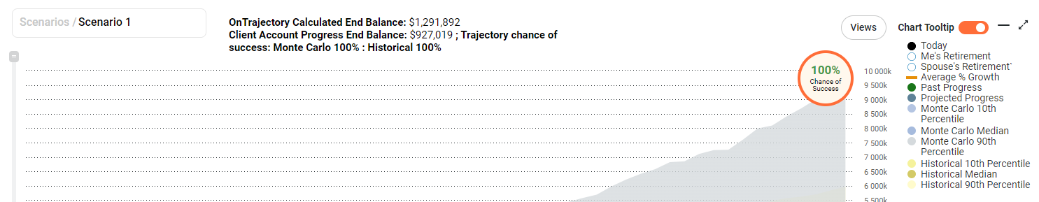
7. Calculate Success % / Chance of Success
Your 'Chance of Success' (located on the top right side of the chart) automatically runs both Historical and Monte Carlo analysis every time you log-in. OnTrajectory then averages the results and displays your 'chance of success'. Success means NOT RUNNING OUT OF MONEY! Anytime you make a data change in the Income, Expenses and Accounts tab, the chart will automatically update with the data change but the ‘Chance of Success’ percentage will not. The reason for this is that running both the Historical and Monte Carlo analysis can be taxing and not every client will want this updated after every data change. But anytime you want to see it updated, just press the ‘Chance of Success’ button and it will start the analysis. You will see 2 percentages displayed on the top of the chart after the analysis is complete. One for Monte Carlo and one for Historical Analysis. The average of these two percentages is what makes up the Chance of Success percentage.
Could your Trajectory End Balance be negative, but your chance of success be quite high? It absolutely could. Remember, your Trajectory is based on Income, Expenses, and the % Growth set for each Account. Analysis is based on returns actually achieved in the past, albeit randomized over time. Could an end balance be positive, but yield a low chance of success? Yes — that would indicate you've set your % Growth assumptions a bit too high.